

Determination of the diffusion coefficient of an inserted species in a host electrode with EIS, PITT and GITT techniques Battery – Application Note 70
Latest updated: June 10, 2024Abstract
The diffusion coefficients of the inserted species are key parameters that determine the battery cell properties. The larger the diffusion coefficient value is, the faster or, more correctly, the more facile the insertion/desinsertion of the inserted species is, and eventually, the better the battery performance is.
Chronoamperometry and chronopotentiometry are classical techniques used to measure diffusion coefficient in the case of a semi-infinite linear diffusion [1-3]. In the case of bounded diffusion, several techniques and analyses are available such as Levich analysis and EIS fitting with the Winf element. Impedance analysis can also performed on commercial Li-ion batteries to try to derive information of the diffusion coefficient of the inserted species.
In this note we will first present the methods to obtain the diffusion coefficient in the case of a system where a restricted linear diffusion reaction is involved, using results from Electrochemical Impedance Spectroscopy (EIS), Galvanostatic Intermittent Titration Technique (GITT) and Potentiostatic Intermittent Titration Technique (PITT) experiments.
Determination of the diffusion coefficient of an inserted species in a host electrode with EIS, PITT and GITT techniques
Introduction
The main electrochemical reaction in a battery intercalation electrode such as an Li-ion battery is the insertion reaction.
In the case of a direct Li+ insertion, the equation, as a reduction reaction, writes:
$$\text{Li}^+ +\text{e}^- + \langle \, \rangle \rightleftharpoons\langle \text{Li} \rangle\tag{1}$$
With $\langle \, \rangle$ an empty insertion site, and $\langle \text{Li} \rangle$ an inserted $Li$ ion within the host material.
The sketch below (Fig. 1) shows the linear insertion or linear restricted diffusion of $\langle \text{Li} \rangle$ in a thin film electrode of a thickness $\text{Li}$.

Figure 1: Schematic of a direct insertion reaction in a thin film electrode, under restricted linear diffusion conditions. The reaction is a reduction reaction that occurs in positive electrode during discharge or negative electrode during charge.
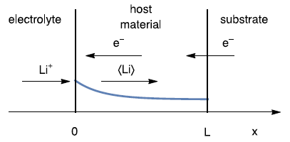
This mechanism is chosen because it can model, in a simple way, the electrochemical process taking place during the insertion and desinsertion of a species into a thin host material.
The blue curve is the concentration of $\langle \text{Li} \rangle$ within the host material. At a length $\text{Li}$, which is the host material thickness:
$$J_{\langle \text{Li} \rangle}=0 \tag{2}$$
With $J_{\langle \text{Li} \rangle}$ the diffusion flux of $\langle \text{Li} \rangle$.
The diffusion coefficients of the inserted species are the key parameters that determine battery cell properties. The larger the diffusion coefficient value is, the faster or rather the more facile the insertion/desinsertion of the inserted species is, and eventually, the better the battery performance is.
Chronoamperometry and chronopotentiome-try are tradiotional techniques used to measure diffusion coefficient in the case of a semi-infinite linear diffusion [1-3]. In the case of bounded diffusion, several techniques and analyses are available such as Levich analysis [4] and EIS fitting with the element [5]. Impedance analysis can also performed on commercial Li-ion batteries to try to derive information concerning the diffusion coefficient of the inserted species [6].
In this note we will first present the methods to obtain the diffusion coefficient in the case of a system where a restricted linear diffusion reaction is involved, using results from Electrochemical Impedance Spectroscopy (EIS), Galvanostatic Intermittent Titration Technique (GITT) and Potentiostatic Intermittent Titration Technique (PITT) experiments.
We will then present some results and analyses obtained on a supercapacitor, which show the typical behaviour associated to a linear restricted insertion, and on an AC Dummy Cell for BCS, which represents the typical behaviour of a two-electrode Li-ion battery cell.
The limits of the described methods and the conditions in which they should be applied will also be made clear.
Measurement methods
EIS
For an electrode, the impedance of the restricted diffusion process has the following expression [7]:
$$Z_\text{M}(f)=R_\text{d}\frac{\text{coth}\sqrt{\tau_\text{d}j2\pi f}}{\sqrt{\tau_\text{d}j2\pi f}}\tag{3}$$
With $\tau_\text{d}$ the diffusion time constant in s, and $R_\text{d}$ the diffusion resistance in Ω, associated with the restricted linear diffusion mechanism.
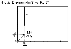
The Nyquist graph of such impedance is shown in Fig. 2: the impedance curve is at higher frequencies a straight line making an angle of -π/4 with the real axis as can be seen with the Warburg element and at lower frequencies a vertical line, similar to a capacitor.
Fitting the graph with the expression shown in Eq. 3 will give access to both $\tau_\text{d}$ and $R_\text{d}$. These two parameters can otherwise be determined by using the characteristic frequency $f_\text{c}$, also named knee-point [8].
$$f_\text{c}=\frac{3.88}{2\pi\tau_\text{d}}=\frac{3.88D_\text{X}}{L^2}\tag{4}$$
With $D_\text{X}$ the diffusion coefficient of the species X in a given medium, and L the thickness of this medium, as defined in Fig. 1.
We also have:
$$\text{Re}({Z_f}_\text{c})=-\text{Im}({Z_f}_\text{c})=\frac{R_\text{d}}{3}\tag{5}$$
Where $\text{Re}({Z_f}_\text{c})$ and $-\text{Im}({Z_f}_\text{c})$ are the real part and the imaginary part, respectively, of the impedance at the characteristic frequency $f_\text{c}$.

Figure 2: Nyquist diagram of the impedance of the M element, characteristic of the linear restricted diffusion.
The faradaic impedance $f_\text{f}$ of the reaction described in Eq. 1 is :
$$Z_\text{f}(f)=R_\text{ct}+Z_\text{M}(f)\tag{6}$$
With $R_\text{ct}$ the charge transfer resistance.
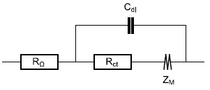
The electrode impedance also comprises a resistance in series as well as a capacitor in parallel to account for the ohmic contribution of the electrolyte and other components and the double layer capacitance, respectively.
A typical electrical equivalent circuit for a host material electrode and its interface within a battery cell is given below (Fig. 3a) as well as a typical Nyquist graph of its impedance (Fig. 3b) [7].
a)
b)
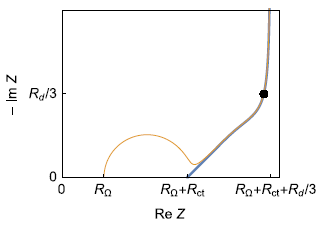
Figure 3: a) Equivalent circuit for the direct insertion reaction in a thin film electrode, under restricted linear diffusion conditions; b) Typical Nyquist graph (black dot : characteristic frequency fc; Blue curve : Zf + RΩ, orange curve: Z).
As it can be seen in Fig. 3, the addition of a charge transfer resistance, an ohmic resistance and a double layer capacitance in parallel does not lead to a more complicated determination of the coefficient diffusion or diffusion time constant : the knee-point frequency or the fitting results can readily lead to it.
A better way of saying this is that, whether the insertion reaction is reversible ($R_\text{ct}\lt \lt R_\text{d}$) or neither reversible nor irreversible ($R_\text{ct}\approx R_\text{d}$), which is the case in Fig. 3b, the diffusion time constant can be determined.
In the case of an irreversible reaction ($R_\text{ct}\lt \lt R_\text{d}$), since diffusion is not the limiting step, the determination of the diffusion time constant is not relevant. Furthermore, the absence of a knee-point frequency makes it more difficult to determine the diffusion time constant, especially if the measurements are noisy.
A more complete description of the diffusion impedances can be found in the Diffusion Impedances Handbook [7].
This typical shape of the impedance diagram of the insertion processes can be found in many recent publications [8-13].
In case the low frequency part of EIS data do not show a knee-point but only a 45 ° angle, it is advised to perform a measurement at lower frequencies. In this case, it might be useful to check the NSD indicator and possibly correct the effect of the time-variance of the system on your data [14,15].
PITT
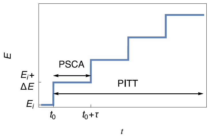
This technique consists of applying a succession of potential steps of constant height as described in Fig. 4a. The PSCA (Potential Step ChronoAmperometry) consists in applying one single step (Fig. 4a). The typical current response is shown in Fig. 4b.
a)
b)
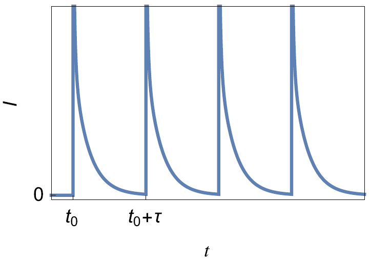
Figure 4: a) Principles of the PITT and PSCA techniques b) Typical current response.
If we consider a reversible insertion reaction (ie. a low charge transfer resistance), no ohmic drop, no double layer capacitance, no phase transitions, a linear restricted diffusion mechanism and finally, a potential step of small amplitude, the diffusion coefficient of a guest species can be determined either from the short-time expression of the diffusion current (Cottrel relationship) or from the long-time domain where an exponential decay of current is predicted [16-19].
- The short-time or Cottrell relationship:
$$I_\text{d}(t)_\text{st}=\frac{FA\sqrt{D}\Delta c}{\sqrt{\pi t}}\tag{7}$$
- The exponential decay at long times:
$$I_\text{d}(t)_\text{It}=-2FA\frac{D}{L}\Delta c \,\text{exp}\left(-\frac{\pi^2Dt}{4L^2}\right)\tag{8}$$
With, $F$ the Faraday constant, $A$ the interfacial surface area, $D$ the diffusion constant of the guest species, $L$ the thickness of the host electrode, $\Delta c$ the variation of guest species concentration due to the potential step, $t$ the time.
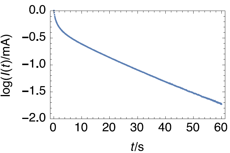
Taking the decimal logarithm of both sides in Eq. (8) and plotting $\text{log}|I(t)|\, v.s. \, t$, the diffusion time constant can be obtained from the slope $\text{SI}_{I_\text{lt}}$ of the portion of straight line (Fig. 5), using the following relationship:
$$\tau_\text{d}= \frac{\pi^2}{4\,\text{ln}10\, \text{SI}_{I_\text{lt}}}\tag{9}$$

Figure 5 : Semi-logarithmic representation of the time current response of a supercapacitor, assuming it behaves as a one electrode system, to a potential step.
From the time constant we can obtain the diffusion coefficient $D$, knowing the electrode thickness $L$:
$$\tau_\text{d}=\frac{L^2}{D}\tag{10}$$
Again, this procedure is only valid when the impedance graph of the concerned electrode only shows a knee-point at low frequency (Fig. 2).
If there is a non-negligible charge transfer resistance, an ohmic resistance and double layer capacitance, Eq. (9) can be used but will only lead to an apparent diffusion or time constant. A different equation could be calculated but would require numerical tools [20].
Warning
Applying this method on a full battery cell with two electrodes will lead to the determination of an average apparent diffusion or time constant. A three-electrode setup is needed to separately study the positive or the negative electrode.
GITT
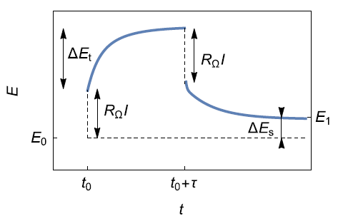
As first described by Weppner and Huggins [2], the GITT technique consists of applying a succession of current steps as with the one illustrated in Fig. 6.
a)
b)![b) Potential response with ∆E_t, the total transient voltage change of the cell for a current I_0for the time τ and ∆E_s the change of the steady-state voltage (from [5]).](data:image/svg+xml;base64,PHN2ZyB4bWxucz0iaHR0cDovL3d3dy53My5vcmcvMjAwMC9zdmciIHdpZHRoPSIzNDIiIGhlaWdodD0iMjQ3IiB2aWV3Qm94PSIwIDAgMzQyIDI0NyI+PHJlY3Qgd2lkdGg9IjEwMCUiIGhlaWdodD0iMTAwJSIgc3R5bGU9ImZpbGw6I2NmZDRkYjtmaWxsLW9wYWNpdHk6IDAuMTsiLz48L3N2Zz4=)
![b) Potential response with ∆E_t, the total transient voltage change of the cell for a current I_0for the time τ and ∆E_s the change of the steady-state voltage (from [5]).](https://biologic.net/wp-content/uploads/2024/06/an70f6a.png)
Figure 6: a) Schematic illustration of a single step of the Galvanostatic Intermittent Titration Technique (GITT) ; b) Potential response with , the total transient voltage change of the cell for a current for the time and the change of the steady-state voltage (from [5]).
Assuming a negligible ohmic drop and a small $I_0$ current step (to ensure the linear behaviour of the system) the diffusion coefficient of the inserted species can be determined with the following relationship [2,3,21]:
$$D=\frac{4}{\pi\tau}\left(\frac{I_0V}{zFA}\right)^2\left(\frac{\Delta E_\text{s}}{\Delta E_\text{t}}\right)^2\tag{11}$$
With $V$ the molar volume of the insertion material, $z$ the number of exchanged electrons in the reaction, $F$ the Faraday constant, $A$ the surface of the electrode/electrolyte interface.
Another method is to adopt the same strategy as for PITT, that is to say to consider the response at longer times.
Using numerical techniques and again provided that the influence of interfacial kinetics and Ohmic potential drop is disregarded, the potential response of a reversible insertion reaction to a current step writes [22]:
$$\Delta E_\text{t}=R_\text{d}I_0\left(\frac{1}{3}+\frac{t}{\tau_\text{d}}-\frac{2}{\pi^2}\sum^\infty_{k=1}\frac{1}{k^2}\exp\left(-k^2 \pi^2\frac{t}{\tau_\text{d}}\right)\right) \tag{12}$$
Which simplifies at long times:
$$\Delta E_{t,\text{lt}}=\frac{R_\text{d}I_0}{3}+\frac{R_\text{d}I_0t}{\tau_\text{d}}\tag{13}$$
With $I_0$ the current step, and $\Delta E_{t,\text{lt}}$ the potential response at long times. $R_\text{d}$ and $\tau_\text{d}$ have the same meaning as in Eq. 3.
According to Eq. 13, plotting $\Delta E_t \, v.s. \, t$, we can measure the slope at long times:
$$|\text{SI}_{E_\text{lt}}|= \frac{R_\text{d}I_0}{\tau_\text{d}}\tag{14}$$
And the ordinate at the origin:
$$\text O_0= \frac{R_\text{d}I_0}{3}\tag{15}$$
Combining Eqs. 14 and 15, it gives:
$$\tau_\text{d}=3\frac{\text O_0}{|\text{SI}_{E_\text{lt}}|}\tag{16}$$
Experimental results
Tested and testing devices
For the sake of simplicity and robustness, we chose to perform measurements on :
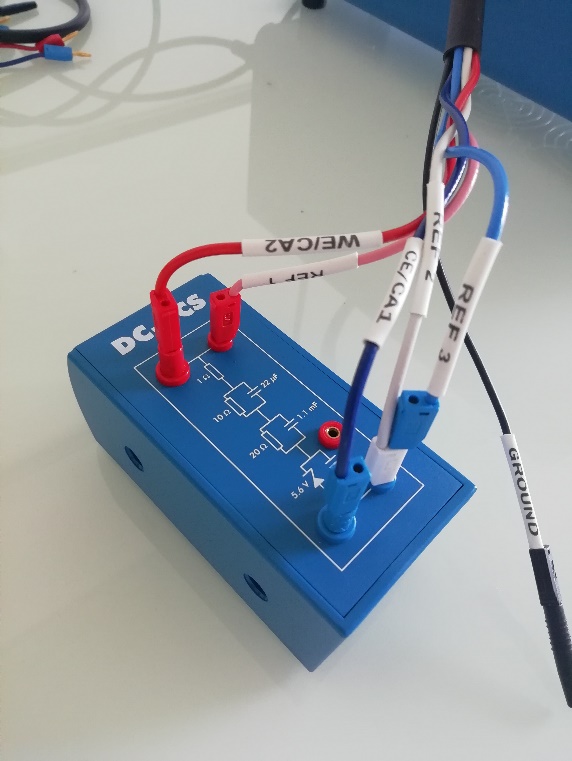
a) a TOKIN supercapacitor of 1 F and max voltage of 5.5 V that is used in the AC dummy cell for the battery cyclers series BCS-805, BCS-810 and BCS-815 (Fig. 7).

Figure 7: Modified AC BCS dummy cell to allow connection on the TOKIN 1 F supercapacitor only
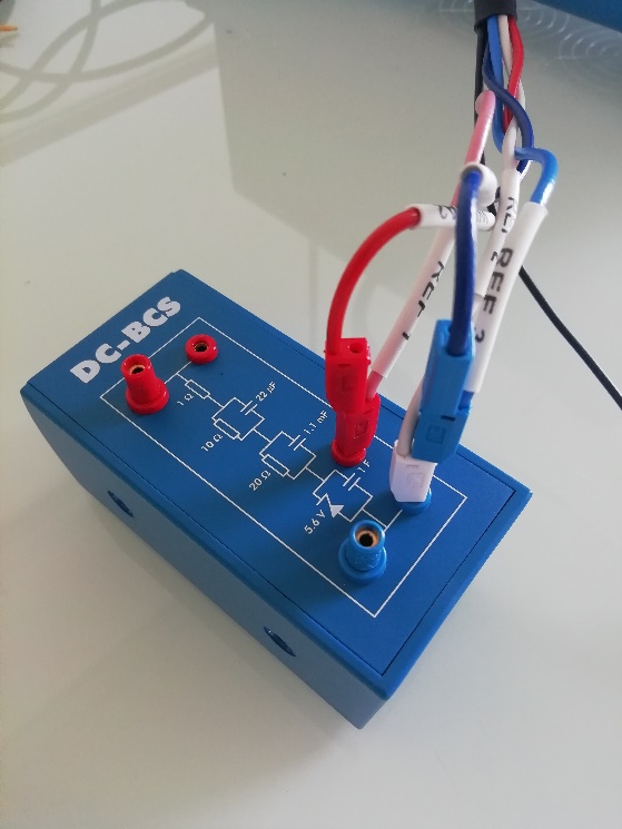
b) the Dummy Cell provided with the BCS to test EIS capability and is composed of a series resistance and two RC’s in series with the above-mentioned supercap (Fig. 8):

Figure 8: Modified AC BCS dummy cell to allow connection on the TOKIN 1 F supercapacitor only
A BioLogic VMP3 potentiostat was used to perform the measurements, except for the measurements with ohmic drop compensation where a BioLogic SP-300 potentiostat was used. The necessity of using the BioLogic SP-300 potentiostat is explained in the Appendix.
Results
a) EIS
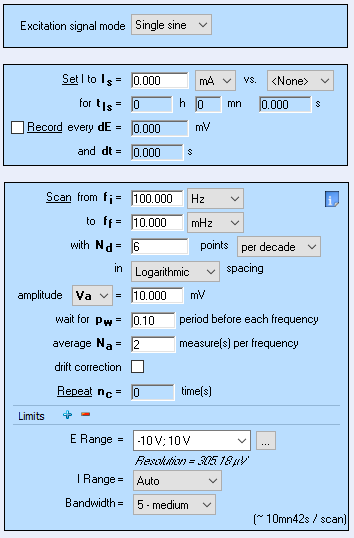
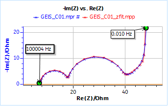
Figure 9 shows the Nyquist diagram of the impedance data obtained on the Tokin 1 F supercapacitor using the GEIS technique with adaptive amplitude (GEIS-AA). The conditions of the experiment are shown in Figure 10.
It can be seen on the impedance graph in Fig. 9 that although the supercapacitor is made of two electrodes where the insertion reactions occur in opposite direction, it behaves as if there was only one insertion reaction, that can be characterized by one single diffusion time constant.

Figure 9: Connection on the modified battery cycler BCS series dummy cell. The nominal values of the components are: R1 = 1 Ω; C1 = 22 µF ; R2 = 10 Ω; C2 = 1.1 mF ; R3 = 20 Ω ; C3 = 1 F
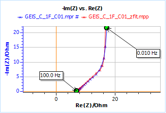

Figure 10 : Nyquist impedance diagram obtained on a Tokin 1 F 5.5 V supercapacitor with the fitting results.
Fitting the results using Z Fit and an R1 + M1 equivalent circuit give the following values for the parameters:
R1 = 7.04 Ω; Rd1 = 29.2 Ω; td1 = 22.3 s
The presence of a series resistance is due to the fact that this is not an ideal supercapacitor. Figure 11 shows the results obtained on the full AC dummy cell for BCS and the fitting results in red.

Figure 11: Parameters of the GEIS technique used to obtain the results in Figure 8.
Using an R1 + R2/C2 + R3/C3 + M1 equivalent circuit and Z Fit, we obtain the following parameters values:
R1 = 7.35 Ω; C2 = 16.0 µF; R2 = 10.5 Ω; C3 = 1.05 mF; R3 = 20.1 Ω; Rd4 = 29.0 Ω; td4 = 22.1 s
We can see that we obtain very close values with both systems for the series resistance R1, the diffusion resistance Rd and the diffusion time constant td.
At low frequencies, the element M is equivalent to the circuit R + C with:
$$R=R_\text{d}/3\tag{17}$$
and
$$C=\tau_\text{d}/R_\text{d}\tag{18}$$
which gives the results shown in Table I.
Parameters values measured by EIS at low frequencies
| Parameters values | τd/s | R/Ω | C/mF | |
|---|---|---|---|---|
| TOKIN Supercap | 22.3 | 9.73 | 763 | |
| Dummy cell AC BCS | 22.1 | 9.67 | 762 |
The capacitance values obtained are very close to each other and not so far from the nominal value, which is 1 F. This shows that the time constant values as measured by EIS are correct.
To conclude, it can be seen that the diffusion kinetic parameters can be quite easily obtained by EIS, independently from the presence of ohmic drop, additonal capacitances and charge transfer resistances.
b) PITT
A potential step of 10 mV was applied on the supercapacitor for 1 min (Fig. 12). The results are shown in Figure 13.

Figure 12: Nyquist impedance diagram obtained on the Dummy Cell AC for BCS with the fitting results.
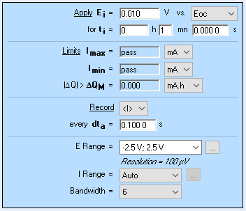
Figure 13 shows the logarithm of the current response of the supercapacitor submitted to a 10 mV potential step. The curve follows an affine law at long times. The initial potential of the supercap was 0.985 V.
The slope given by the Linear Fit tool is – 0.0263 s-1, which, using Eq. 9 gives a time constant of 40.7 s.
Using an ohmic compensation technique to account for the presence of a series resistance allows users to obtain a different slope of – 0.0399 and a time constant of 26.9 s, closer to the value obtained by EIS. Please see Appendix for the results as well as the corresponding BioLogic application notes [23-25].

Figure 13 : Parameters used to perform the PITT (PSCA) experiment on the supercapacitor and the dummy cell AC BCS.
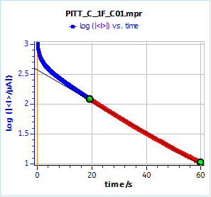

Figure 14: Decimal logarithm of the current response of the TOKIN supercapacitor to a 10 mV potential step with the Linear Fit tool in EC-Lab® to calculate the slope.
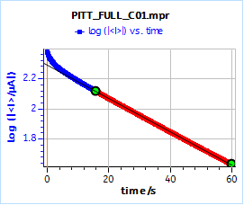
Figure 14 shows the current response of the full AC BCS dummy cell to a 10 mV potential step. The slope obtained using the EC-Lab® Linear Fit tool is -0.011 s-1, which gives a time constant of 97.4 s, very far from the value obtained by EIS. This shows that Eq. 5 is only valid for systems where there is no ohmic drop, no additional capacitances and charge transfer resistances.
Using ohmic drop compensation, we find a time constant of 85.8 s, which is a little better but still far from the value found by EIS.
Figure 14: Decimal logarithm of the current response of the TOKIN supercapacitor to a 10 mV potential step with the Linear Fit tool in EC-Lab® to calculate the slope.
c) GITT
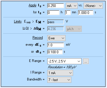
Figure 15 shows the potential response of the TOKIN supercap to an ascending and then descending 250 µA current step. The control parameters of the step are given in Fig. 16. The linear fit tool gives us the value of the slope of the potential response at long times and the ordinate at the origin, 0.313 mV/s and 1061.0 mV, respectively. The ordinate at the origin must be corrected by the initial potential value 1 057.2 mV. Using Eq. 16, this gives a time constant of 36.4 s.

Figure 15: Decimal logarithm of the current response of the full BCS AC dummy cell to a 10 mV potential step with the Linear Fit tool in EC-Lab® to calculate the slope.
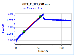

Figure 16: Potential response of the TOKIN 1 C supercap to an ascending and descending 250 µA current step.
The plot shown in Fig. 15 could be corrected from the ohmic drop. The ohmic or series resistance can be calculated using the method described in Fig. 6.
The ohmic drop is equal to , where and are the second and first potential values on the curve, respectively.
The corrected curve is shown in Fig. 17 (obtained using Excel):

Figure 17: Parameters of the current step used to obtain the potential response shown in Figs. 15 and 17.
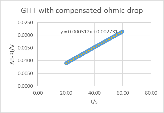
Using the the equation of the trendline and Eq. 16, it gives a time constant of 26.3 s. Correcting from the ohmic drop gives a value of the time constant, that is close to the one obtained with EIS and PITT
We can perform the same analysis on the results obtained on the full dummy cell.

Figure 18: Potential response from Fig. 16 subtracted from the initial potential and the ohmic drop RI
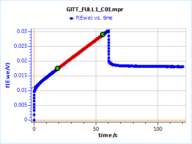
The slope is 0.315 mV/s and the ordinate at origin 0.0115 V, which gives a time constant of 110.0 s, which, as for PITT, is also overrated.
We can measure the ohmic drop which corresponds to the potential value of the second point in Fig. 18: 1.89 mV.
The compensated curve is shown in Fig. 19 (obtained using Excel). Again, using the slope and the ordinate at origin as well as Eq. 16 gives a time constant of 91.7 s, which is still far from the EIS value but yet a little bit closer than without compensation.

Figure 19: Potential response difference ΔE of the AC BCS dummy cell to an ascending and descending 250 µA current step.
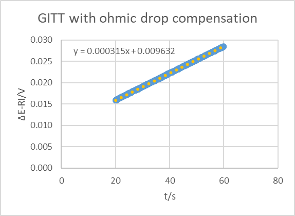
Table II below shows a summary of the values obtained for the time constants in s with each method. The values highlighted in green are correct. The ones highlighted in yellow are almost correct and the values in highlighted in red are far from being correct.
Diffusion time constants in s obtained on the TOKIN supercap and the AC-BCS dummy cell for each method.
| Method | Supercap | AC dummy cell |
|---|---|---|
| EIS | 22.3 | 22.1 |
| PITT | 40.7 | 97.4 |
| PITT (RI) | 26.9 | 85.8 |
| GITT | 36.4 | 110.0 |
| GITT (RI) | 26.3 | 91.7 |
Conclusion
In this note, DC and AC methods to obtain the diffusion time constants were presented. From the results shown in Table II it seems clear that, considering a single electrode:
- Only EIS can give access to the a correct value of the time constant, when the studied system is not reversible and has non-negligible capacitances and charge transfer resistances.
- If the system is reversible but has a series resistance, methods to compensate this series resistance are proved to be somewhat efficient.
- The simple and classical equations (Eqs. 9 and 16) that can be used with PITT and GITT techniques to provide diffusion time constants and coefficients are only applicable when the system is a single electrode, where a totally reversible insertion reaction takes place with negligible charge transfer resistances and double layer capacitances.
If the system is composed of several charge transfer resistances and double layer capacitances, for example an electrode in a battery cell, or the full battery cell, composed of two electrodes, numerical methods are required to derive the right temporal equations [20].
References
1) A. J. Bard, L. R. Faulkner, Electrochemical Methods, Fundamentals and applications, Wiley, New York (1980)
2) W. Weppner, R. Huggins, J. Electrochem. Soc., 124, 110 (1977) 1569.
3) C. Wen, B. Boukamp, R. Huggins, W. Weppner, J. Electrochem. Soc., 126, 12 (1979) 2258.
4) BioLogic Application Note 56
5) BioLogic Application Note 66
6) BioLogic Application Note 61
7) J.-P. Diard, B. Le Gorrec, C. Montella Handbook of Diffusion Impedances
8) T. Zhang, B. Fuchs, M. Secchiaroli, M. Wohlfahrt-Mehrens, S. Dsoke, Electrochim. Acta 218 (2016) 163.
9) S. Brown, N. Mellgren, M. Vynnycky, G. Lindbergh, J. Electrochem. Soc., 155, 4 (2008) 320.
10) S. Malifarge, B. Delobel, C. Delacourt, J. Electrochem. Soc., 164, 11 (2017), 3329.
11) M. Oldenbürger, B. Bedürftig, A. Gruhle, F. Grimsmann, E. Richter, R. Findeisen, A. Hintennach, J. Energy Storage 21 (2019) 272.
12) S. Song, X. Zhang, C. Li, K. Wang, X. Sun, Y. Wa, J. Power Sources 490 (2021) 229332.
13) X. Zhang, X. Zhang, X. Sun, Y. An, S. Song, C. Li, K. Wang, F. Su, C.-M. Chen, F. Liu, Z.-S. Wu, Y. Ma, J. Power Sources 488 (2021) 229454.
14) BioLogic Application Note 64
15) BioLogic Application Note 69/2
16) C. Montella, J. Electroanal. Chem., 518, 2 (2002) 61.
17) C. Montella, Electrochim. Acta, 51, 15 (2006) 3102.
18) C. Montella, J. Electroanal. Chem., 633, 1 (2009) 35.
19) C. Montella, J. Electroanal. Chem., 633, 1 (2009) 45.
20) C. Montella, R. Michel, J.-P. Diard, J. Electroanal. Chem., 608, 1 (2007) 37.
21) E. Markevich, M. Levi, D. Aurbach, J. Electroanal. Chem., 580 (2005) 231.
22) C. Montella, J.-P. Diard, J. Electroanal. Chem., 623 1 (2008) 29.
23) BioLogic Application Note 27
Appendix
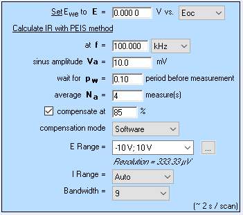
To perform the PITT measurements with compensated series resistance, we used the ZIR technique to measure the ohmic drop. It consists in an EIS measurement at a single frequency. Although it is a better method than current interrupt (CI) it is not ideal, especially in the case where high frequency inductance is not negligible, as can be seen in batteries. This aspect is better explained in BioLogic Application Note 29 [25].
Also, it was necessary to use the smallest potential range available giving the smallest resolution, that is to say 1 µV, such that the correction does not trigger large current drops. This potential range also requires the use of BioLogic Premium range instruments, ie in this case SP-300 potentiostat. Figures 20 and 21 show the parameters and the results, respectively.
a)
b)
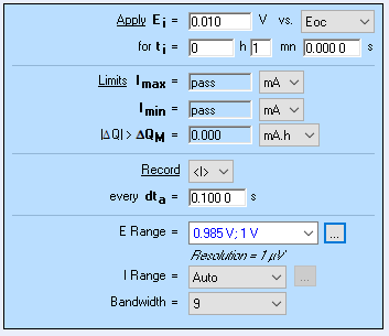
Figure 20: a) ZIR parameters and b) CA parameters used to obtain the PITT curves with compensated ohmic resistance shown in Fig. 21
a)
b)
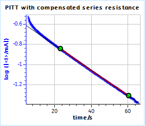
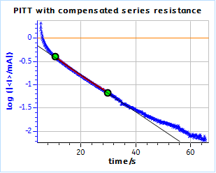
Figure 21: PITT curves with series resistance compensation for a) the TOKIN supercapacitor and b) the AC BCS dummy cell. The ohmic resistance was measured by ZIR technique.
Scientific articles are regularly added to BioLogic’s Learning Center:
To access all BioLogic’s application notes, technical notes and white papers click on Documentation:
https://biologic.net/documents/
Latest revision: June 15th 2021


