

How to read EIS accuracy contour plots Electrochemistry & Battery – Application Note 54
Latest updated: May 28, 2024Abstract
The impedance measurement accuracy of an impedance analyzer depends on both the impedance magnitude and the measurement frequency. The EIS specifications for potentiostats/galvanostats are given in a graph called a contour plot. The aim of this note is to help users understand and use the EIS accuracy contour plots so as to recognize and interpret possible errors in their EIS measurements.
Introduction
The impedance measurement accuracy of an impedance analyzer depends on the impedance magnitude and on the measurement frequency. Potentiostats/galvanostats/Impedancemeters specifications are given in graphs called accuracy contour plots1. The aim of this note is to help the user understand and use EIS accuracy contour plots.
Contour Plot

Figure 1: 3D graph of a two-variable function, level curve (blue curve) and projection in the x, y plan (red curve).
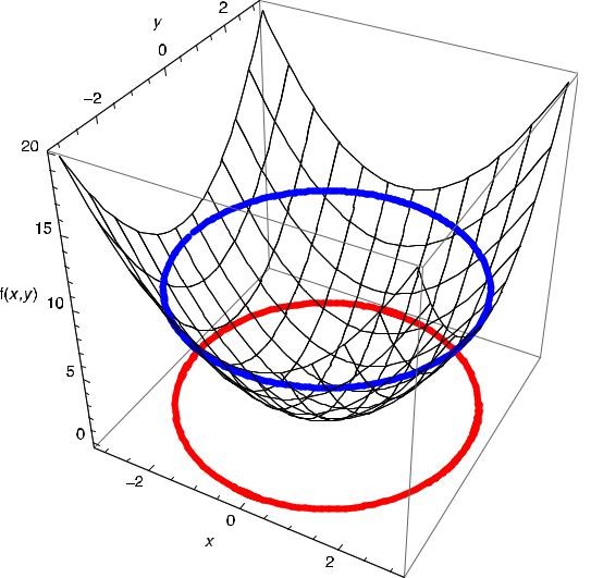
Contour plots are isovalue curves of a function depending on two variables. As an example 3D graph of a two variables function f(x, y) = x2 + y2 and a level curve of this function for f(x, y) = 10 are shown in Fig. 1. The level curve is a cross-section of the 3D graph parallel to the (x, y) plan at f(x, y) = 10. The projection of this curve on the x, y plane is a contour plot. For any point (x, y) inside of this contour, we have f(x, y) < 10 and for any point outside of this contour we have f(x, y) ≥ 10.
EIS Accuracy Contour Plot
SP-300 EIS Accuracy Contour Plot
The scheme of an EIS accuracy contour plot is shown in Fig. 2.

Figure 2: Scheme of an EIS accuracy contour plot.
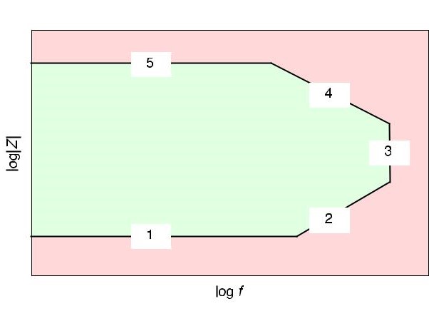
The two horizontal limits (high (5) and low (1) Z) are related to the ability of the instrument to accurately measure/control the current. To increase the high Z portion of accuracy contour plot, the instrument has to be able to measure low current (often related to the electrometer impedance in the specifications).
To increase the low part of the accuracy contour plot, the instrument has to be able to manage high current. A current booster may be added to improve the measurement in this area. The vertical limit (3) depends on the regulation speed of the instrument. This is the maximum frequency that can be reached by the instrument with an acceptable error. It is related to the bandwidth of the instrument. The two other limits (4) and (2) are related to stray capacitor and stray inductor, respectively. Inductive effects are very sensitive to current levels and the cell connections.
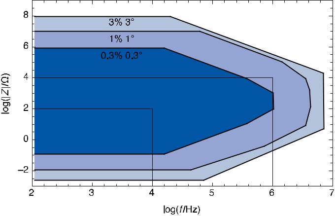
The contour plot of an SP-300 potentiostat is shown in Fig. 3. The shaded areas show different ranges of impedances that can be measured at various frequencies within a specified error in magnitude and in phase. These errors refer to the borders and not to the areas as explained below.

Figure 3: SP300 EIS accuracy contour plot. Black dot: f = 106 Hz, |Z| = 104 Ω, white dot: f = 104 Hz, |Z| = 102 Ω.
Example
Let us consider the black dot in Fig. 3. This dot corresponds to the measurement of an impedance |Z| = 104 Ω measured at a frequency f = 106 Hz. As this measurement is located between the 0.3 %, 0.3◦ and 1 %, 1◦ contour plots, the accuracy is 0.3 % < |Z|/|Z| < 1 %, for the modulus (relative error) and 0.3◦ < φZ < 1◦ for the phase (absolute error). The phase is given in absolute error because the relative error could be indeterminate in the case where φ = 0. An impedance whose modulus is 100 Ω at 104 Hz is measured with a relative uncertainty lower than 0.3 % for the modulus and lower than 0.3◦ for the phase (Fig. 3, white dot).
How to Use an EIS Contour Plot
Impedance of the R1+R2/C2 Circuit
The impedance for the R1+R2/C2 is given by
$$Z(f)=R_1+ \frac{R_2}{1+R_2C_2j2\pi f}\tag{1}$$
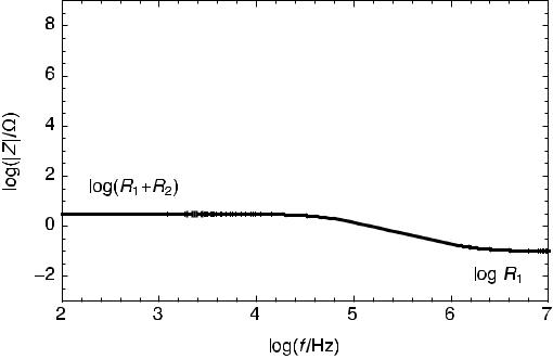
The modulus of the impedance as a function of the frequency is shown in Fig. 4 for R1 = 0.1 Ω, R2 = 3 Ω and C2 = 10−6 F.

Figure 4: Modulus Bode diagram of the impedance for the R1+R2 /C2 circuit. R1 = 0.1 Ω, R2 = 3 Ω and C2 = 10– 6 F.
Example #1
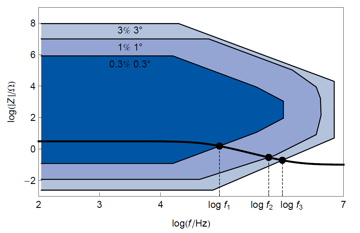
The modulus Bode impedance diagram of this electrical circuit R1+R2/C2 and the SP-300 contour plot are superimposed in Fig. 5. This figure allows us to predict the precision of the impedance measurements as a function of frequency. One has to determine the frequency values where the modulus diagram moves into a different precision domain. For instance, the modulus diagram moves from the high precision domain (|Z|/|Z| < 0.3 % and φZ < 0.3◦) to the mid-range precision domain (0.3 < |Z|/|Z| <1 % and 0.3 < φZ < 1◦) for a frequency moving from f1 ≈ 10 kHz to f2 ≈ 60 kHz (Fig. 5).

Figure 5: Superimposition of the modulus Bode impedance diagram of the electrical circuit R1+R2/C2 and the SP-300 contour plot.
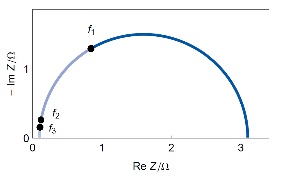
The Nyquist impedance diagram of the R1+R2/C2 circuit is shown in Fig. 6 with the impedances measured at f1, f2 and f3.

Figure 6: Nyquist diagram of the impedance for the R1+R2 /C2 circuit, f1 ≈ 10 kHz, f2 ≈ 60 kHz, f3 ≈ 100 kHz.
Tab. I shows how the precision of the impedance modulus and phase evolves with the frequency for the R1+R2/C2 electrical circuit with intermediate Rs and C values.
Table I: Impedance measurement accuracy as a function of the frequency. R1 = 0.1 Ω, R2 = 3 Ω and C2 = 10−6 F.
| Frequency | Impedance modulus | Impedance phase |
|---|---|---|
| $$f \lt f_1$$ | $$\Delta|Z|/|Z| \lt 0.3\% $$ | $$\phi_Z \lt 0.3°$$ |
| $$f_1 \lt f \lt f_2$$ | $$0.3\% \lt \Delta|Z|/|Z| \lt 1\% $$ | $$ 0.3° \lt \Delta \phi_Z \lt 1°$$ |
| $$f_2 \lt f \lt f_3$$ | $$1\% \lt \Delta|Z|/|Z| \lt 3\% $$ | $$ 1° \lt \Delta\phi_Z/° \lt 3°$$ |
| $$f \gt f_4 $$ | $$\Delta|Z|/|Z| \gt 3\% $$ | $$ \phi_Z \gt 3°$$ |
Example #2
Another situation can be observed for high values of R2 and low values of C2, for instance R1 = 104 Ω, R2 = 0.2 × 10⁷ Ω and C2 = 5 × 10⁻⁹ F (Figs. 7 and 8).

Figure 7: Superimposition of the modulus Bode impedance diagram of the electrical circuit R1+R2/C2 (high Rs values and low C value) and the SP-300 contour plot.
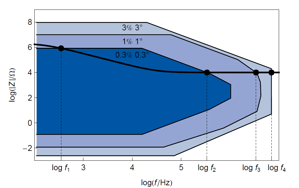

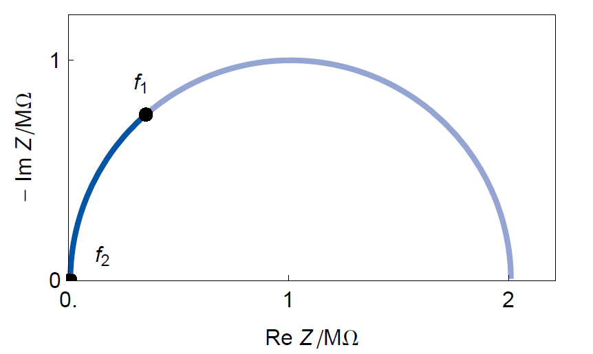
Figure 8: Nyquist diagram of the R1+R2/C2 circuit. R1= R1 = 104 Ω, R2 = 0.2.107 Ω and C2 = 5.10-10 F.
As the frequency reaches lower values, measurement precision moves outside of the best precision domain. Tab. II shows how the precision of the impedance modulus and phase, evolves with the frequency for an R+R/C electrical circuit with high R values and low C values.
Tab. II: Change of impedance measurement accuracy with frequency. R1 = 104 Ω, R2 = 0.2 × 10⁷ Ω and C2 = 5 × 10⁻¹⁰ F.
| Frequency | Impedance modulus | Impedance phase |
|---|---|---|
| $$f \lt f_1$$ | $$0.3\% \lt \Delta|Z|/|Z| \lt 1\% $$ | $$0.3° \lt \Delta \phi_Z \lt 1°$$ |
| $$f_1 \lt f \lt f_2$$ | $$\Delta|Z|/|Z| \lt 0.3\% $$ | $$\Delta \phi_Z \lt 0.3°$$ |
| $$f_2 \lt f \lt f_3$$ | $$1\% \lt \Delta|Z|/|Z| \lt 3\% $$ | $$ 1° \lt \Delta \phi_Z \lt 3°$$ |
| $$f \gt f_4 $$ | $$\Delta|Z|/|Z| \gt 3\% $$ | $$ \Delta \phi_Z \gt 3°$$ |
Conclusion
This note aims to explain how to read and understand EIS contour plots, which are provided with each of our instruments. Contour plots must be used to interpret errors made during EIS measurements and identify the best frequencies possible to be used for a given impedance range.
Appendix
Definitions [1]
Measurand:
Quantity intended to be measured, quantity subject to measurement.
Measurement accuracy:
Closeness of agreement between a measured quantity value and a true quantity value of a measurand. The concept `measurement accuracy’ is not a quantity and is not given a numerical quantity value. A measurement is said to be more accurate when it offers a smaller measurement error.
Measurement uncertainty, uncertainty:
Non-negative parameter characterizing the dispersion of the quantity values being attributed to a measurand.
Measurement precision, precision:
Closeness of agreement between indications or measured quantity values obtained by replicate measurements on the same or similar objects under specified conditions.
References
1) International vocabulary of metrology. Basic and general concepts an associated term. JCGM (2008).
Revised in 07/2018
[1] Considering the definitions given in [1] and recalled in Appendix A, the word accuracy is a time-honored misnomer. Uncertainty should preferably be used.


