

EIS Quality Indicators: THD, NSD & NSR Battery & Corrosion – Application Note 64
Latest updated: May 22, 2024Abstract
Three quality indicators are available in EC-Lab® to quantitatively assess the quality and the validity of your EIS experiment, the EIS QI™ include: i) Total Harmonic Distortion quantifies the linearity of the response, ii) Non Stationary Distortion indicates the effect of time-variance and transient regime, finally iii) Noise to Signal Ratio ensures the signal is large enough compared to the measurement noise. Some results are given on the electrical circuit as well on a discharging battery.
Introduction
EIS is a powerful technique used to study an electrochemical system in a specific state and understand the nature of the reactions occurring at the interface. Usually, this technique is based on the analysis of the linear response of an electrochemical system submitted to a potential or current sinusoidal modulation.
For an EIS experiment as defined above to be valid, the system under study should fulfill various requirements:
- The system should be linear. A simple example of a linear system is a resistor [1].
- The response of the system should not be transient i.e. it should have reached a steady-state or permanent regime [2].
- The values of the parameters defining the system should not change throughout the experiment. Impedance measurements on a time-variant system can lead to a wrong interpretation [3].
- The system should be the same throughout the experiment. For example, a passive electrode that depassivates is not an adequate system.
Most electrochemical systems have a non-linear behavior. Nonetheless, when submitted to a modulation of a small amplitude, their behavior can be considered as linear. The value of this amplitude depends on the characteristics of the system, so for each system, we need a way to ensure that the chosen amplitude is small enough. This is the role of the first EIS QI™: the Total Harmonic Distortion (THD).
Furthermore, it should be ensured that the system and its response does not change throughout the experiment. A parallel can be made with photography: the object that is being shot should not be moving during the opening time of the shutter. There is a second indicator that is made available for that: the Non Stationary Distortion (NSD) indicator.
Additionally, another indicator is made available and is related to the quality of the signal: the Noise-to-Signal Ratio (NSR). It ensures that the input modulation is not too low and that the amplitude of the response is significant compared to the response measurement noise.
In this application note, we will first present how these indicators are calculated and then show results that illustrate their use.
Theoretical Description
In this part of the note we will briefly explain the indicators.
For more theoretical information please refer to EC-Lab® User’s Manual.
Total Harmonic Distortion (THD)
As already stated in the introduction, most of the electrochemical systems are non-linear. By applying an input signal of small amplitude, non-linear systems can be considered as linear.
The THD indicates if the amplitude of the current or potential modulation applied to the system is small enough to consider that it behaves linearly. If a system behaves non-linearly the output signal will contain some harmonics. The THD quantifies the non-linearity by evaluating the amplitudes of the N harmonics:
$$\text{THD}_\text N=\frac{1}{|Y_f|} \sqrt{\sum_{k=2}^N |Y_k|^2}\tag{1}$$
where |Yf| is the amplitude of the signal at the fundamental frequency f (or first harmonic) and |Yk| is the amplitude of the kth harmonic number.
THD is expressed as a percentage. Generally, it is considered that a THD below 5% is acceptable. In EC-Lab®, it is calculated on the potential and on the current and over 6 harmonics (N = 7).
For more details about linearity and non-linearity of systems please see [1].
Non-Stationary Distortion (NSD)
As mentioned in the introduction, it is important that the system and its response do not change with time during an impedance measurement.
We can distinguish two causes for the non-stationarity of a system: i) the response of the system has not reached its permanent regime; ii) the parameters defining the system are changing with time.
The response of a non-stationary system will contain, in addition to the fundamental frequency, some adjacent frequencies.
Hence the NSD indicator is defined as:
$$\text{NSD}_{\Delta f}=\frac{1}{|Y_f|} \sqrt{|Y_{f-\Delta f}|^2 + |Y_{f+\Delta f}|^2}\tag{2}$$
where |Yf| is the amplitude of the signal at the fundamental frequency f (or first harmonic), |Yf-Δf| et |Yf+Δf| are the amplitudes of the peaks right next to the fundamental frequency and Δf is the frequency resolution
The NSD is expressed as a percentage and calculated on the potential and current. The drift correction in EC-Lab® is based on the compensation of the adjacent frequencies [2].
Noise to Signal Ratio (NSR)
In an ideal measurement, all the signal energy is contained in the fundamental frequency, but because of various factors such as the accuracy and precision of the measuring device or external perturbations, there might be some energy in other frequencies than the fundamental one, which is called noise.
The NSR quantifies the extent of noise in the measurement. It is expressed using the following formula:
$$\text{NSR}_{f}=\frac{1}{|Y_f|} \sqrt{\sum_{k} |Y_{k\Delta f}|^2}\tag{3}$$
with:
$k\Delta \notin \{f; 2f; 3f; 4f; 5f; 6f; 7f; f-\Delta f; f+\Delta f\}$
It represents all the signal not contained in:
- The fundamental frequency,
- The 6 harmonics used to calculate THD
- The signal at frequencies adjacent to the fundamental frequency used to calculate NSD. Some results will now be shown to illustrate these indicators.
Results on Electrical Circuits
The measurements were performed on the Test Box-3. This is a series of electrical circuits made by BioLogic that mimics typical behaviours of electrochemical systems. The first circuit is a a linear system, the second and third ones are non-linear systems and mimic a Tafel and a passivating system, respectively [1]. To active the EIS quality indicator option you need to go to “Advanced Settings” in EC-Lab®.
TEST BOX-3 #1: A Linear System
As can be seen in Fig. 1, the DC response of the electrical circuit corresponding to Test Box-3 #1 is linear.

Figure 1: Steady-state response of Test Box-3 #1. Scan rate: 20 mV/s.
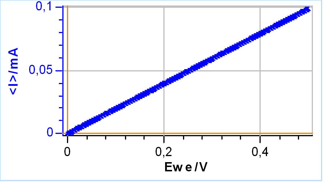
Figure 2 shows Nyquist diagrams of measurements made at various amplitudes. They were performed using one channel of a BP-300 with a low current option. The detailed parameters are shown in the Appendix Fig. A1.

Figure 2: Nyquist diagrams of EIS measurements performed on Test Box-3 #1 using increasing amplitudes: 2, 5, 10, 13, 15, 20 mV. Frequency range: 100 kHz – 1 Hz.
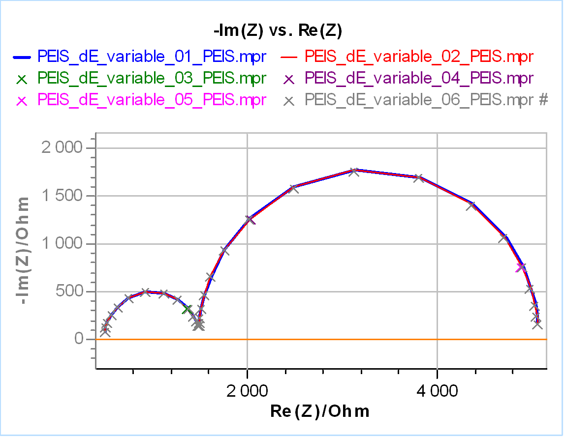
It can be seen that whatever the amplitude the Nyquist diagram is the same. These diagrams can be fitted using an R1 + R2/C2 + R3/C3 electrical equivalent circuit. The results of the fit are given in Tab. A1. The normalized standard deviation (σ/mean) of the six measurements does not go over 0.21%, showing that the impedance does not depend on the input amplitude. Figure 3 shows the THD on the current (THD I) for all six measurements.

Figure 3: THD of the current during EIS measurements performed on Test Box-3 #1 using increasing amplitudes: 2, 5, 10, 13, 15, 20 mV. Frequency range: 100 kHz – 1 Hz.
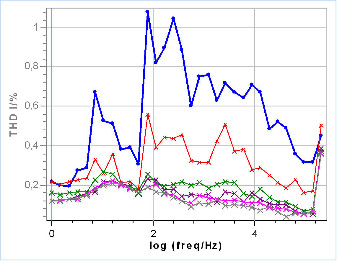
The value of the THD on the current is never over 1% and decreases, surprisingly, with increasing amplitudes. This can be explained using Eq. 1: as the amplitude of the potential modulation is increased, the amplitude of the fundamental frequency Yf also increases while the amplitudes of the harmonics – that are only due to measurement noise – stay identical. Consequently, THD I decreases with the amplitude.
TEST BOX-3 #2: A Non-Linear System
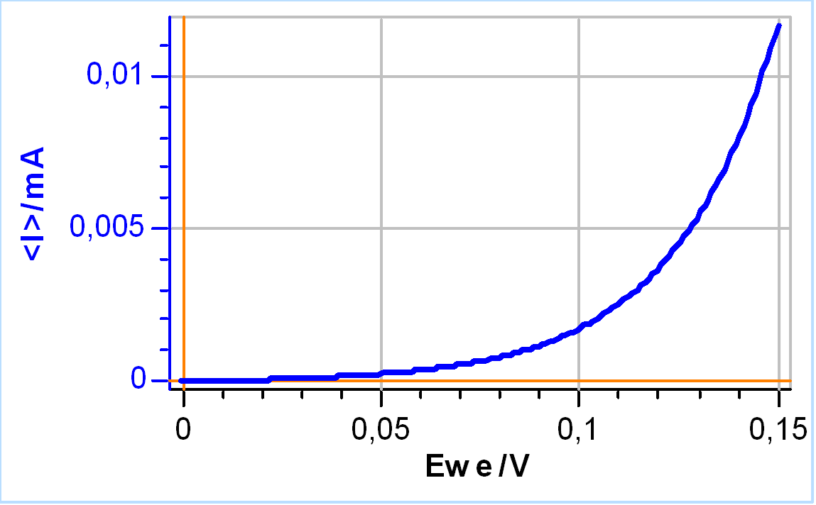
As said above, the Test Box-3 #2 mimics an electrochemical system with a Butler-Volmer or Wagner-Traud, as can be seen in Fig. 4.

Figure 4: Steady-state response of Test Box-3 #2. Scan rate: 20 mV/s.
EIS measurements were then performed at various amplitudes. The detailed parameters are given in Appendix Fig. A1. The results are shown in Fig. 5.

Figure 5: Nyquist diagrams of EIS measurements performed on Test Box-3 #2 using increasing amplitudes: 2, 5, 10, 13, 15, 20 mV. Frequency range: 100 kHz – 1 Hz.
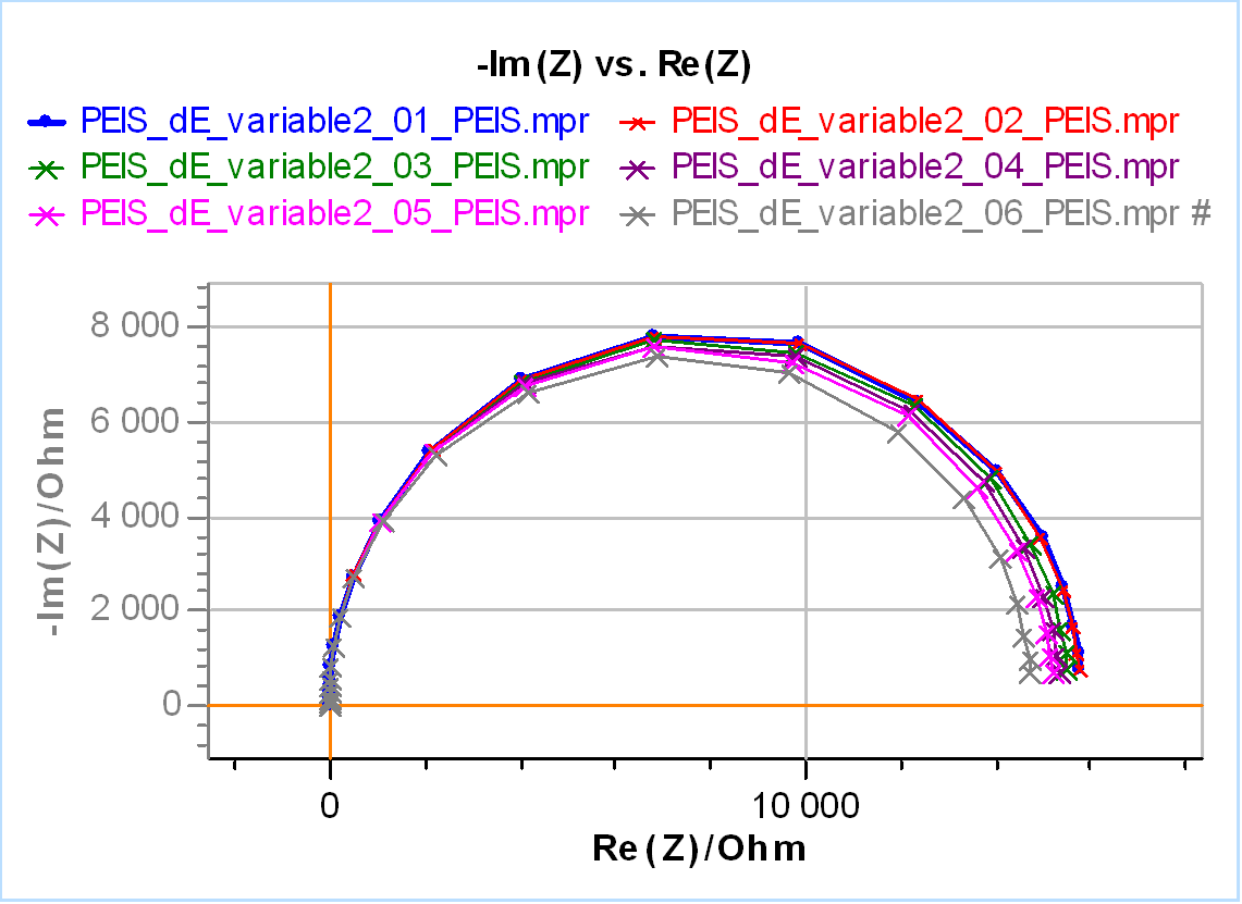
We can see that the Nyquist plots of the impedance change with the amplitude. As the amplitude increases, the impedance modulus at low frequency value decreases. However, this circuit can be fitted using an R/C electrical equivalent circuit. Detailed results of the fitting are given in the Appendix Table AII. The normalized standard deviation of the value of R1 is 2.34%, which shows that the impedance diagram depends on the input modulation amplitude. Figure 6 shows the corresponding THD I.

Figure 6: THD of the current during EIS measurements performed on Test Box-3 #2 using increasing amplitudes: 2, 5, 10, 13, 15, 20 mV. Frequency range: 100 kHz – 1 Hz.
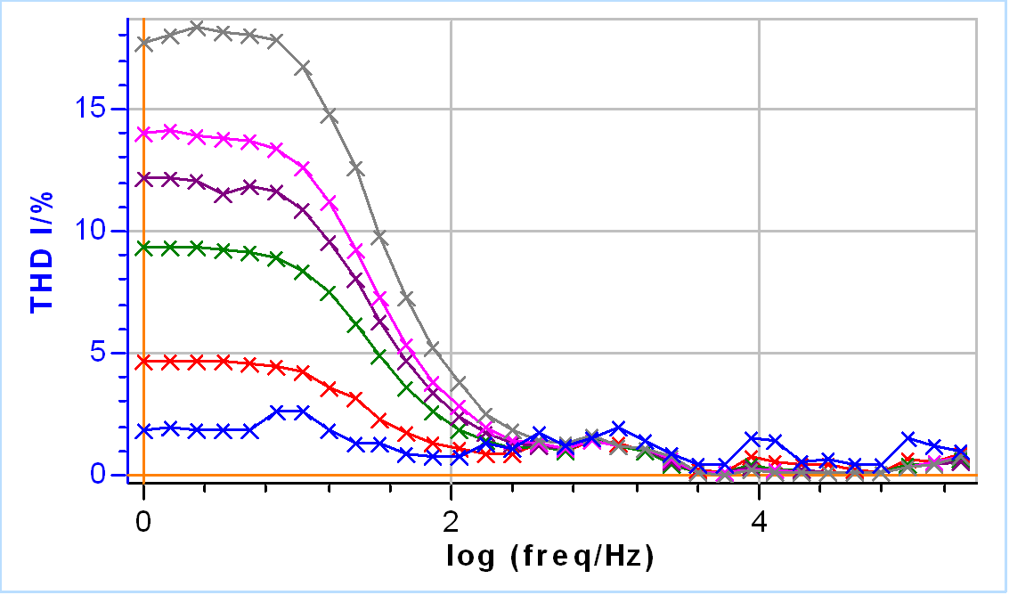
It can be seen that only at 5 mV the THD I is equal to 5%, which can be considered as an acceptable value. Above 5 mV the amplitude is too large as the THD I goes up to 10% for 10 mV and then up to almost 20% for 20 mV. One can also see that the THD I and consequently the non-linear behaviour of the system also depends on the frequency. Using the results shown in Fig. 6, we can adopt a strategy to hide non-linearity, which is to limit the frequency range of our measurements above 100 Hz (log(100) = 2). Above this value, the THD I is always lower than 5% for all chosen amplitudes.
In this particular example the NSD is not relevant as there is no reason why the values of the components of the electrical circuit would change over time (the temperature is controlled in the room where the experiment took place).
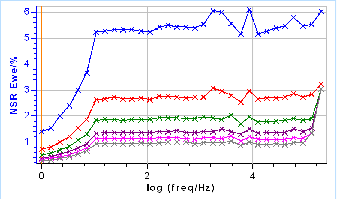
The last indicator that could be used is NSR, which is the sum of the amplitudes of all the frequencies (except the fundamental, the adjacent to the fundamental and the 6 harmonics) divided by the amplitude of the fundamental frequency of the response. In this case it is interesting to take a look at both the NSR E and the NSR I, in Fig. 7a and Fig. 7b, respectively.
Figure 7a shows that the NSR E decreases as the amplitude is increased which is due to the fact that the term Yf is increasing in Eq. 3. At 2 mV, even though the THD I (Fig. 6) indicates it is small enough, it cannot be used for this impedance measurement as it is too small to provide a satisfactory NSR E. An amplitude of 5 mV provides a better NSR E of around 5%.
When considering the NSR I, the effect of using a small amplitude is even more visible as it reaches a maximum of 70%. The saw-shaped signal is explained by auto-ranging. As the current decreases with frequency, the current ranges also decrease. Moving to a lower range increases the accuracy of the measurement and hence reduces the measurement noise and the NSR I.
a)
b)
Figure 7: a) NSR of the potential and b) NSR of the current during EIS measurements performed on Test Box-3 #2 using increasing amplitudes: 2, 5, 10, 13, 15, 20 mV. Frequency range: 100 kHz – 1 Hz.
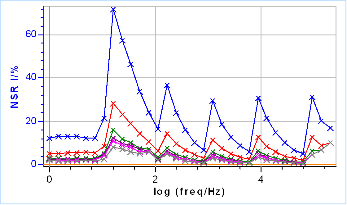
This saw-shaped NSR I could be removed using a fixed current range but this could be highly problematic at lower frequencies as the accuracy of the measuring range compared to the current quantity to be measured would produce an even higher NSR I.
Choosing the right amplitude comes down to a trade-off between non-linearity and noise-to-signal ratio. As can be seen in Fig. 5 and 7b, even a high NSR I does not necessarily mean noisy measurements whereas a THD I as high as 10% can already affect the results.
We will now show some results on a non-stationary system (a discharging battery) to illustrate the NSD quality factor.
Results on a Discharging Battery
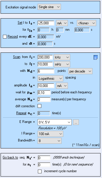
Impedance measurements in galvanostatic mode were performed on a Samsung ICR 18650 commercial battery. Detailed conditions are shown in Appendix Fig. A3.
Two different discharge currents were used:
-20 mA and -25 mA.
The sinusoidal modulation was 10 mA for both currents.
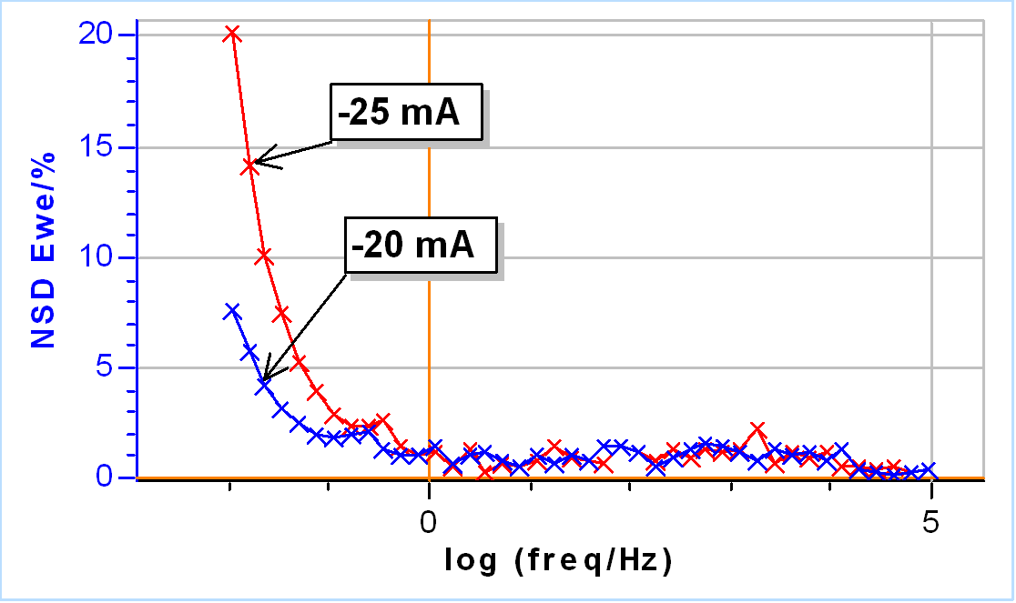
Figure 8a shows the Nyquist plot of the impedance and Figure 8b the resulting NSD on the potential response.
The signal starts to become distorted by non-stationarity at around 1 Hz as is shown in Fig. 8b. For -20 mA discharge current, the NSD E exceeds 5% at 15 mHz. When the discharge current is increased, the NSD E also increases for measurement at the same frequencies because the system is supposed to vary more rapidly with time. In this case the NSD E exceeds 5% at larger frequency i.e. 50 mHz.
a)
b)
Figure 8: a) Nyquist impedance graph and b) corresponding NSD E of commercial 18650 LFP battery at two discharge currents: -20 mA (blue) and -25 mA (red). Modulation amplitude of 10 mA. Frequency range: 100 kHz to 10 mHz.
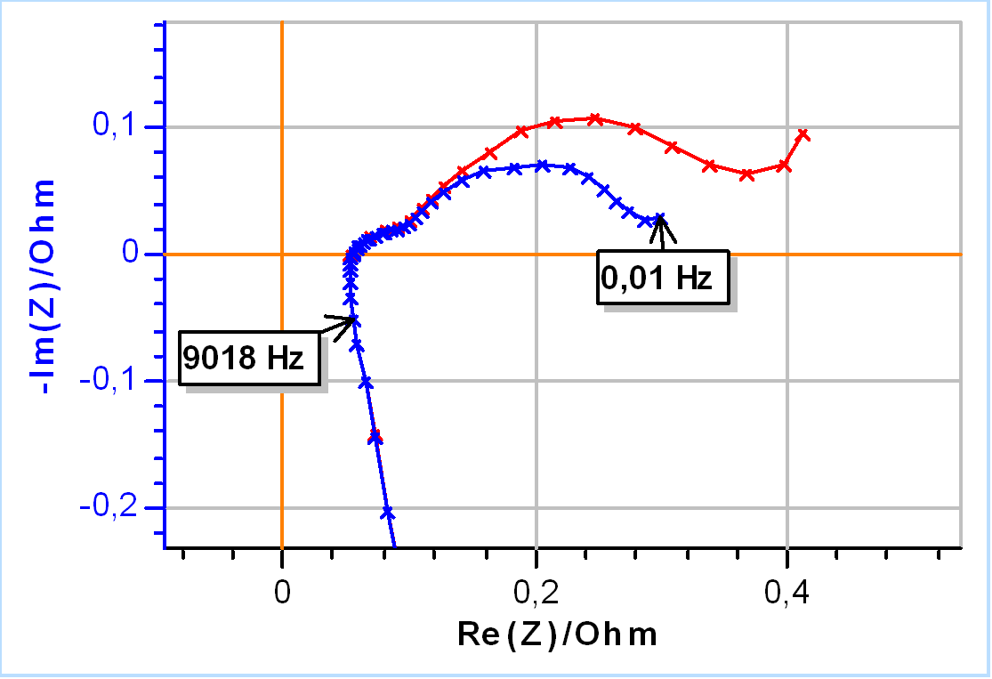
In this case, since the NSD depends on the DC perturbation, the source for non-stationarity is the variation of the system, that is to say its parameters are the same but their values change with time. At higher frequencies, the changes are too slow to affect the measurements.
Conclusion
In this note we introduced three parameters, available since EC-Lab® 11.20, that give quantitative information on the quality of electrochemical impedance measurements and help find the best input parameters.
THD and NSR can be used to optimize the amplitude of the input AC modulation and NSD to optimize the DC perturbation applied to the system.
A small amplitude means a low THD I but also a high NSR E, so this is a compromise. A large potential compared to the OCP will certainly produce a higher NSD I than if only OCV is applied.
These frequency-dependent parameters were illustrated with results obtained on the Test Box-3 and a commercial battery.
Data files can be found in:
C:\Users\xxx\Documents\EC-Lab\Data\Samples\EIS\AN64_
References
1) Application Note #9 “Linear vs. non linear systems in impedance measurements.”
2) Application Note #17 “Drift correction in electrochemical impedance measurements”
3) Application Note #55. “Interpretation problems of impedance measurements made on time-variant systems.”
Appendix

Figure A1: Parameters for the results shown in Figs. 2, 3, 5-7. The same were used for the other amplitudes.
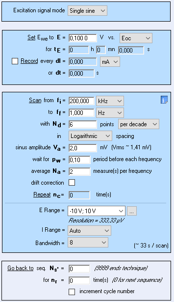
Table AI: Fitting Results of impedance data shown in Fig. 2
| Va/mV | R1/Ω | R2/Ω | C2/nF | R3/Ω | C3/µF |
|---|---|---|---|---|---|
| 2 | 500.3 | 992.3 | 9.78 | 3569 | 2.07 |
| 5 | 500.8 | 990.3 | 9.77 | 3564 | 2.08 |
| 10 | 500.3 | 990.5 | 9.76 | 3555 | 2.08 |
| 13 | 500.5 | 991.5 | 9.74 | 3554 | 2.09 |
| 15 | 500.5 | 991.6 | 9.75 | 3553 | 2.09 |
| 20 | 500.6 | 992.2 | 9.75 | 3554 | 2.09 |
| σ/mean/% | 0.03 | 0.08 | 0.15 | 0.17 | +0.21 |
Table AII: Fitting Results of impedance data shown in Fig. 5
| Va/mV | R1/Ω | C1/nF |
|---|---|---|
| 2 | 15817 | 495.6 |
| 5 | 15797 | 495.7 |
| 10 | 15558 | 495.9 |
| 13 | 15367 | 495.7 |
| 15 | 15224 | 495.6 |
| 20 | 14769 | 495.3 |
| σ/mean/% | 2.34 | 0.04 |

Figure A2: Parameters for the results shown in Figs. 8. The same were used for the other discharge current.
revised 12/2019


