Interpretation problems of impedance measurements on time variant systems Battery & Corrosion – Application Note 55

Introduction

Application note #9 [1] deals with impedance measurements performed on linear (and non-linear) time-invariant systems. Electrochemical systems like a battery in operation or a corroding electrode are rarely time-invariant. Impedance graphs obtained on time-variant systems can often mislead to incorrect interpretation and analysis when using equivalent electrical circuit. This application note describes two examples of such misleading interpretations using a commonly used electrical equivalent circuit with a variable resistor.

Impedance Diagram for Time-Variant System

R1+R2(t)/C2 Circuit with Increasing R2

The time evolution of systems, such as operating batteries or corroding electrodes, is not known a priori and hence cannot be predicted.

Figure 1: R1+R2(t)/C2 circuit.

Let us consider the R1+R2(t)/C2 circuit [2] (ZFit was used to graphically code the circuit) shown in Fig. 1 and assume that the resistance R2 increases with time according to the following relationship:

$$R2(t)=R2_0 + kt^2\tag{1}$$

The impedance was calculated for a measurement carried out with one period of sinusoidal signal. The impedance is calculated at the frequency f_n using the R2 resistance value at time t given by

$$t(f_n)=\sum^n_{i=1}t(f_i)=\sum^n_{i=1}\frac{1}{(f_i)}\tag{2}$$

where t(f_i) is the duration of the measurement of one point on the diagram, i.e. the inverse of the measurement frequency [3].

Figure 2: Instantaneous Nyquist impedance diagrams (t = 0 and t = t_max) of the circuit R1+R2(t)/C2 (R1 = 50 Ω, R2₀ = 500 Ω, k = 10^–5 Ω s^–2, C2 = 2.10^–2 F) and simulation of the measured diagram (•). The dot size increases with increasing time.

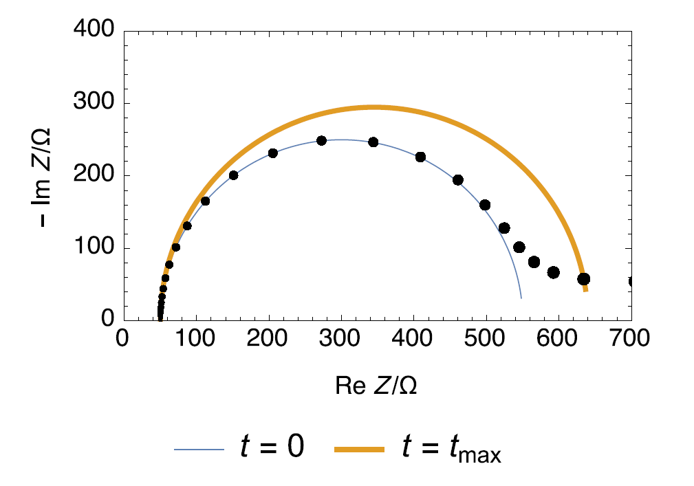
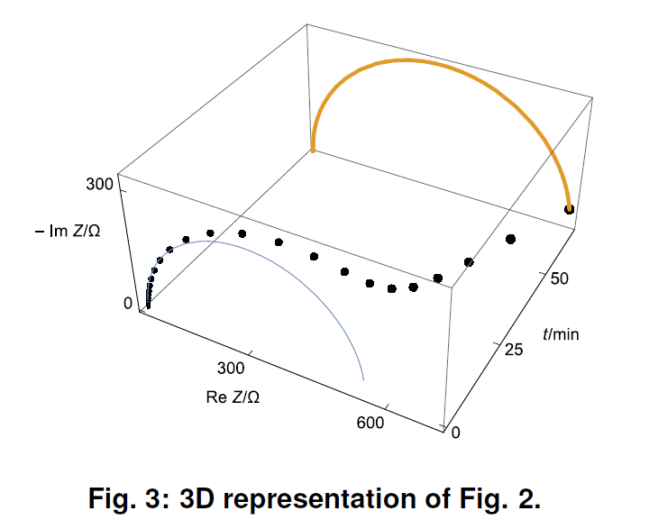
Figure 3: 3D representation of Fig. 2.

The frequency sweep is performed from f_max  ! f_min with f_max  = 10 Hz and f_min  = 10⁻³ Hz. All frequencies are logarithmically distributed over 8 points per decade. The parameters used for R1, R2 and C2 are described in the caption of Fig. 2.

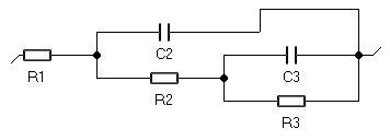
The simulated impedance diagram in Figs. 2 and 3 show the beginning of a low frequency arc. The impedance of the circuit described in Fig. 4 can show a time-invariant Nyquist graph similar to the time-variant Nyquist graph of the circuit shown in Fig. 1.

Figure 4: R1+C2/(R2+C3/R3) circuit.

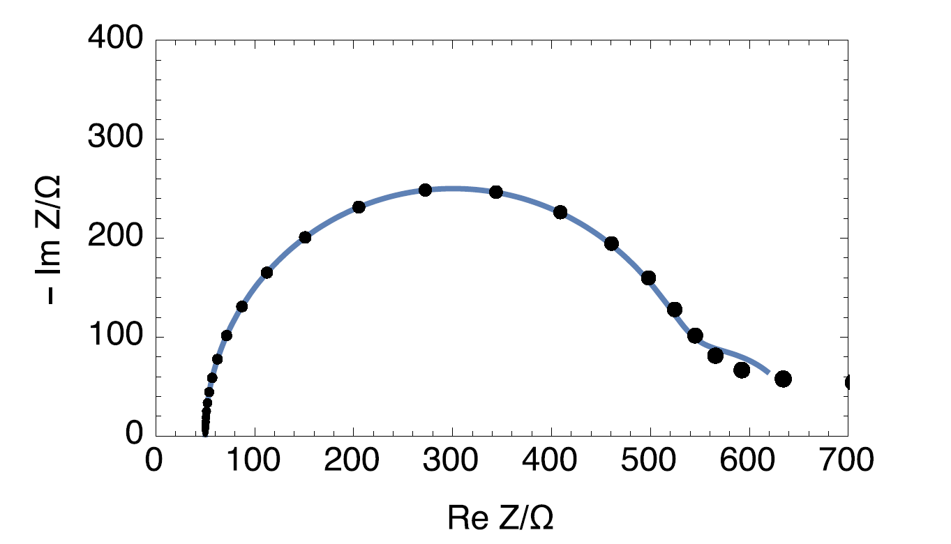
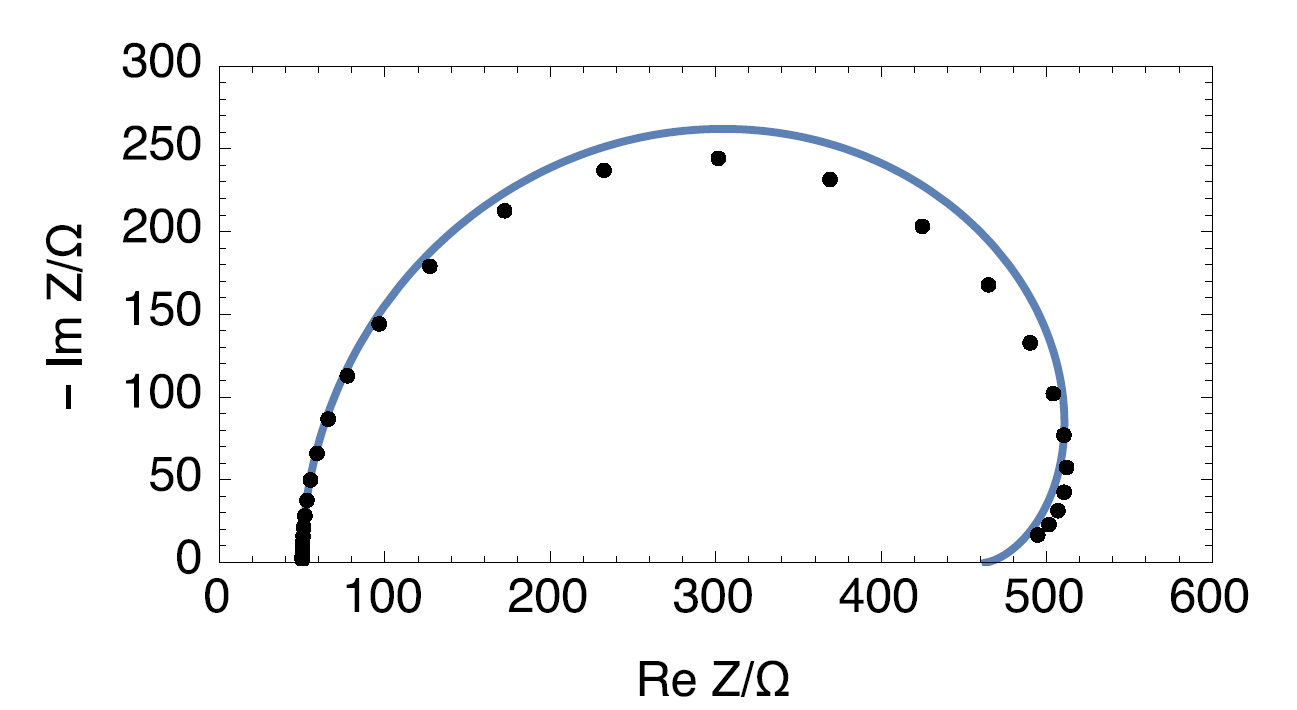
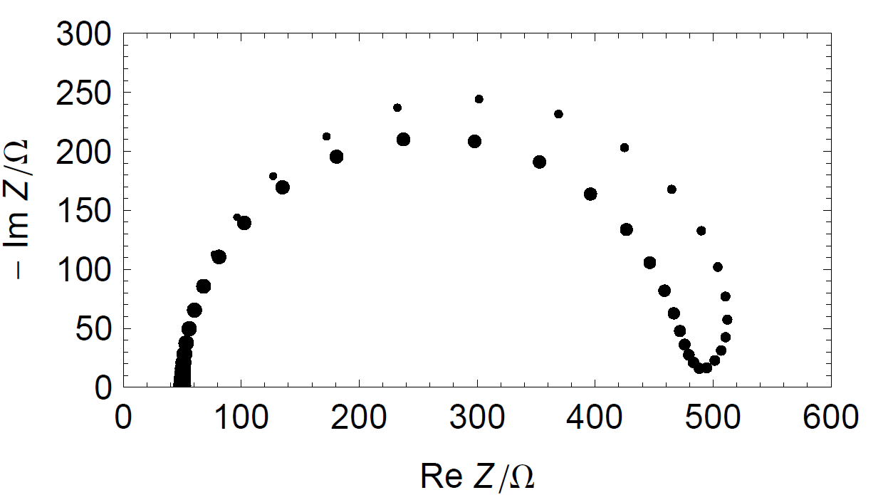
Both graphs are compared in Fig. 5. This shows that a user unaware of the time-variance of the system can mistakenly try to fit the data with a more complicated equivalent circuit than the one required.

Figure 5: Nyquist impedance diagram of the time-variant circuit R1+R2(t)/C2 (•) and Nyquist impedance diagram of the time-invariant circuit R1+C2/(R2+C3/R3), with R1 = 50 Ω, R2 = 500 Ω, C2 =  10² F, R3 = 100 Ω, C3 = 1 F.

R1+R2(t)/C2 Circuit with Decreasing R2

A second case of variation of the resistance R2 is shown in Fig. 6. The value of resistor R2 is henceforth supposed to decrease with time according to

$$R2(t)=R20-k’\sqrt{t}\tag{3}$$

Figure 6: Instantaneous Nyquist impedance diagrams (t = 0 and t = t_max) of the circuit time-variant R1+R2(t)/C2 and simulation of the measured diagram (•).

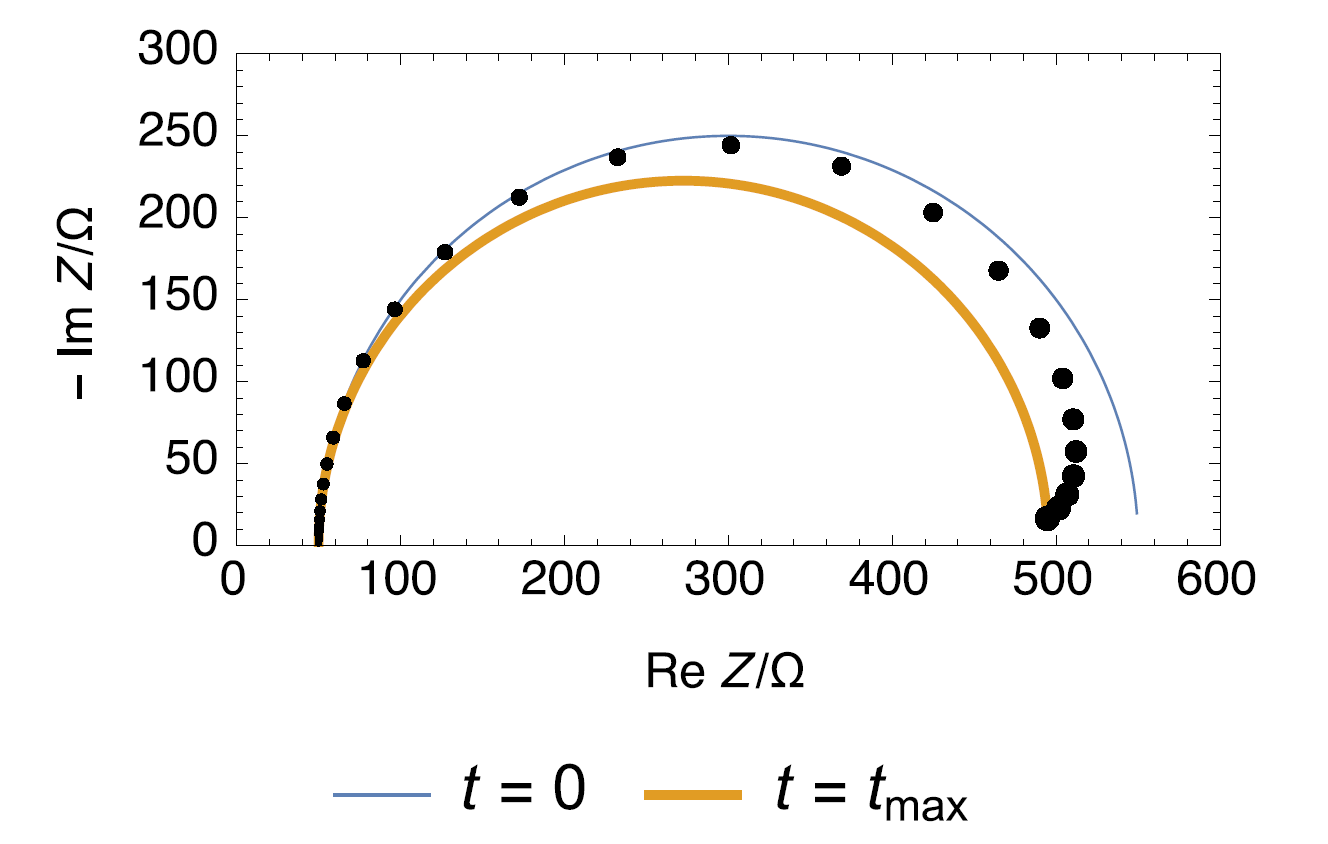
Figure 7: Nyquist impedance diagram of the time-variant circuit R1+R2(t)/C2 (•) and Nyquist impedance diagram of the time-invariant circuit R1+C2/(R2+C3/R3), with R1 = 50 Ω, R2 = 534.375 Ω, C2 = 1.1.10 ² F, R3 = 123.75 Ω, C3 = 0.125 F.

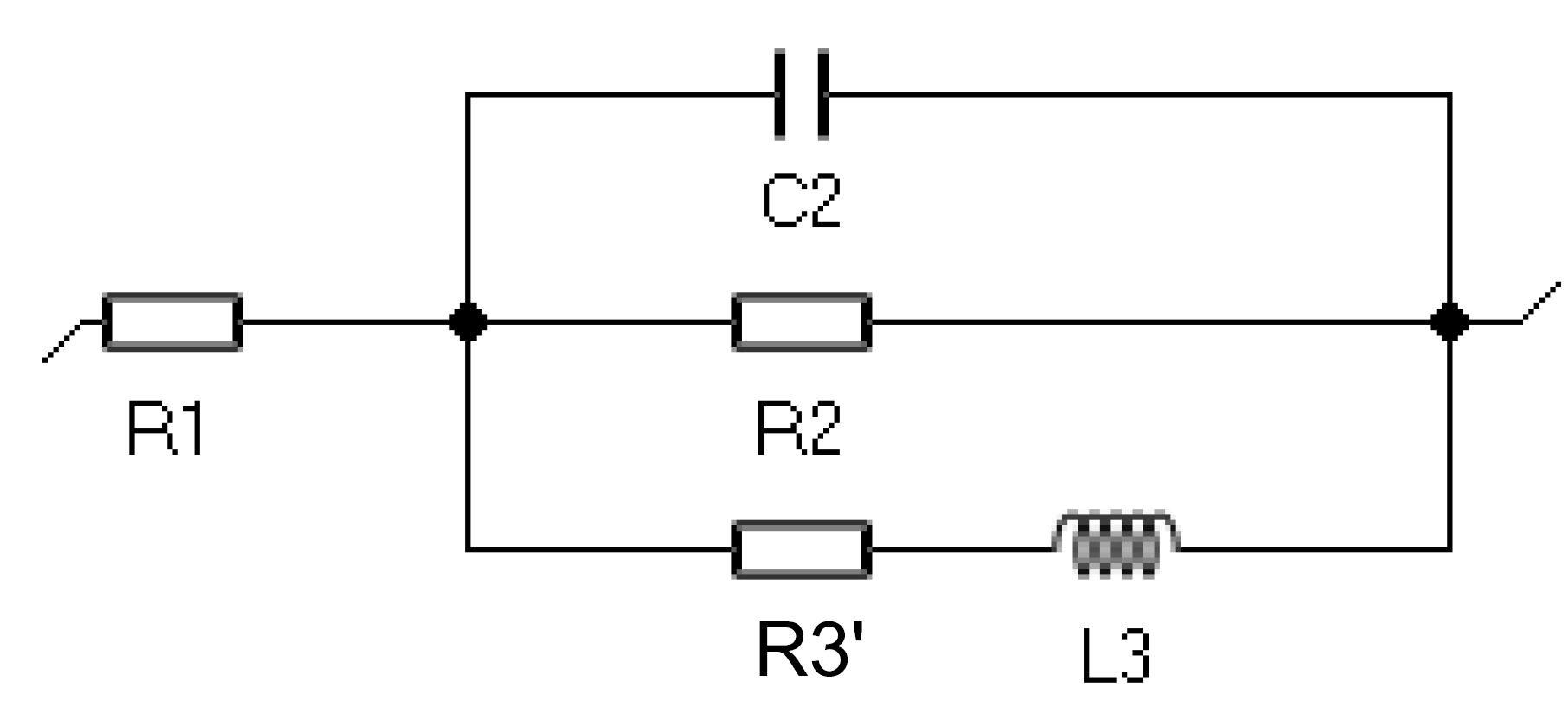
Remember that it is possible to convert the circuit shown in Fig. 4 with R3 < 0 and C3 < 0 to the circuit R1+C2/R2/(R3’+L3) shown in Fig. 8 with R3 > 0 and L3 > 0 where [4]

$$R3’=-\frac{R2(R2+R3)}{R3},L3=-R2^2C3\tag{4}$$

Figure 8: Circuit R1+C2/R2(R3’+L3).

Stationary System Check

Kramers-Kronig (KK) Transforms

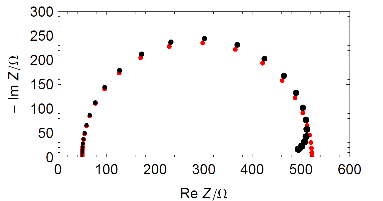
Calculated impedance ZKK using KK transforms is shown in Fig. 9. Nyquist impedance Z and ZKK diagrams are not similar for all frequencies, therefore impedance measurement has not been carried out for a time invariant system [5].

Figure 9: Simulation of the measured Nyquist diagram of the R1+R2(t)/C2 circuit (•) and Nyquist impedance diagram obtained using KK transform (•).

Successive Measurements

A simpler method is to successively perform two identical measurements (Fig. 10). One trick is to successively link two impedance measurements by decreasing frequency f_max   f_min then immediately by increasing frequency f_min  f_max (Fig. 11).

Figure 10: Simulated Nyquist impedance diagram of the circuit R1+R2(t)/C2 for two successive impedance measurements with scan f_max → f_min.

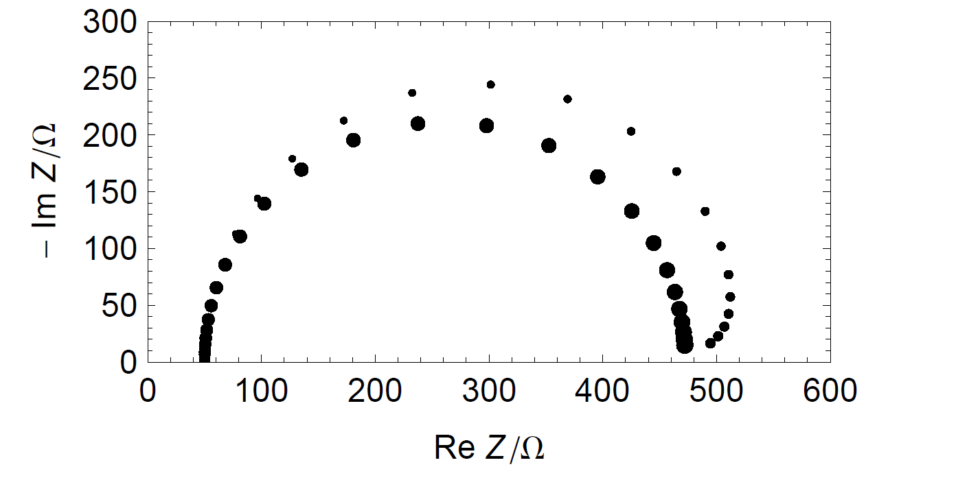
Figure 11: Simulated Nyquist impedance diagram of the circuit R1+R2(t)/C2 and for two successive impedance measurements with scan f_max → f_min → f_max.

The two impedance diagrams shown in Figs. 10 and 11 are different, which proves that the studied system is time variant.

References

1) Application note #9 “Linear vs. non linear systems in impedance measurements.”
2) Z. Stoynov and B. Savova-Stoynov, J. Elec-troanal. Chem. 183 (1985) 133.
3) F. Berthier, J.-P. Diard, A. Jussiaume, and J.-J. Rameau, Corrosion Science 30 (1990) 239.
4) J.-P. Diard, B. Le Gorrec, and C. Montella, Cinetique électrochimique, Hermann, Paris, (1996).
5) Application note #15 “Two questions about Kramers-Kronig transformations.”
Revised in 08/2019